3. Features selections and optimization
3.1. New features
The objective of this part is to create additional feature to improve the algorithm efficiency.
The added features is:
#------------------------------------------------------------------
# Optimize Feature Selection/Engineering
#------------------------------------------------------------------
### Create new feature(s)
EnronDataFrame[myTools.CONST_RATIO_SALARY_TOTAL_PAYEMENTS_LABEL]=EnronDataFrame[myTools.CONST_SALARY_LABEL].combine(EnronDataFrame[myTools.CONST_TOTAL_PAYMENTS_LABEL],func=myTools.ratio)
EnronDataFrame[myTools.CONST_RATIO_BONUS_TOTAL_PAYEMENTS_LABEL]=EnronDataFrame[myTools.CONST_BONUS_LABEL].combine(EnronDataFrame[myTools.CONST_TOTAL_PAYMENTS_LABEL],func=myTools.ratio)
print(str("New feature {}:\n{}").format(myTools.CONST_RATIO_SALARY_TOTAL_PAYEMENTS_LABEL,EnronDataFrame.sort_values([myTools.CONST_RATIO_SALARY_TOTAL_PAYEMENTS_LABEL],ascending=False)[[myTools.CONST_RATIO_SALARY_TOTAL_PAYEMENTS_LABEL,myTools.CONST_SALARY_LABEL,myTools.CONST_TOTAL_PAYMENTS_LABEL]].head(10)))
print()
print(str("New feature {}:\n{}").format(myTools.CONST_RATIO_BONUS_TOTAL_PAYEMENTS_LABEL,EnronDataFrame.sort_values([myTools.CONST_RATIO_BONUS_TOTAL_PAYEMENTS_LABEL],ascending=False)[[myTools.CONST_RATIO_BONUS_TOTAL_PAYEMENTS_LABEL,myTools.CONST_BONUS_LABEL,myTools.CONST_TOTAL_PAYMENTS_LABEL]].head(10)))
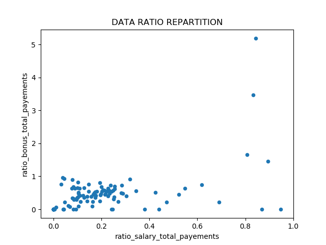
myTools.pyplot_scatter(data=EnronDataFrame,label_x=myTools.CONST_RATIO_SALARY_TOTAL_PAYEMENTS_LABEL,label_y=myTools.CONST_RATIO_BONUS_TOTAL_PAYEMENTS_LABEL,fileName="ratioRepartition.png",show=True,title="DATA RATIO REPARTITION")
print("Selected Features statistics: ")
print(EnronDataFrame.describe().transpose())
# Add new feature to the selected feature list
features_list+=[myTools.CONST_RATIO_SALARY_TOTAL_PAYEMENTS_LABEL,myTools.CONST_RATIO_BONUS_TOTAL_PAYEMENTS_LABEL]
Note
Thanks to these new features, we can observe a potential outlier with very high bonus ratio : HANNON KEVIN P. By exploring database, HANNON KEVIN P is a POI. This graph confirm the new features interest.
3.1.1. ratio_salary_total_payements new feature:
Name |
ratio_salary_total_payements |
salary |
total_payments |
|---|---|---|---|
BERBERIAN DAVID |
0.947950 |
216582.0 |
228474.0 |
DERRICK JR. JAMES V |
0.893633 |
492375.0 |
550981.0 |
REDMOND BRIAN L |
0.868294 |
96840.0 |
111529.0 |
HANNON KEVIN P |
0.842772 |
243293.0 |
288682.0 |
RICE KENNETH D |
0.832860 |
420636.0 |
505050.0 |
ELLIOTT STEVEN |
0.807373 |
170941.0 |
211725.0 |
DODSON KEITH |
0.690762 |
221003.0 |
319941.0 |
TILNEY ELIZABETH A |
0.619285 |
247338.0 |
399393.0 |
CARTER REBECCA C |
0.548226 |
261809.0 |
477557.0 |
JACKSON CHARLENE R |
0.523533 |
288558.0 |
551174.0 |
3.1.2. ratio_bonus_total_payements new feature:
Name |
ratio_bonus_total_payements |
bonus |
total_payments |
|---|---|---|---|
HANNON KEVIN P |
5.196029 |
1500000.0 |
288682.0 |
RICE KENNETH D |
3.465003 |
1750000.0 |
505050.0 |
ELLIOTT STEVEN |
1.653088 |
350000.0 |
211725.0 |
DERRICK JR. JAMES V |
1.451956 |
800000.0 |
550981.0 |
BELDEN TIMOTHY N |
0.954262 |
5249999.0 |
5501630.0 |
ALLEN PHILLIP K |
0.930997 |
4175000.0 |
4484442.0 |
DONAHUE JR JEFFREY M |
0.913492 |
800000.0 |
875760.0 |
KITCHEN LOUISE |
0.893078 |
3100000.0 |
3471141.0 |
HICKERSON GARY J |
0.816603 |
1700000.0 |
2081796.0 |
COLWELL WESLEY |
0.805183 |
1200000.0 |
1490344.0 |
3.1.3. Enron database statistics
feature |
count |
mean |
std |
min |
25% |
50% |
75% |
max |
|---|---|---|---|---|---|---|---|---|
salary |
145.0 |
1.841671e+05 |
1.969598e+05 |
0.0 |
0.0 |
210500.000000 |
2.690760e+05 |
1.111258e+06 |
bonus |
145.0 |
6.713353e+05 |
1.230148e+06 |
0.0 |
0.0 |
300000.000000 |
8.000000e+05 |
8.000000e+06 |
total_payments |
145.0 |
2.243477e+06 |
8.817819e+06 |
0.0 |
91093.0 |
916197.000000 |
1.934359e+06 |
1.035598e+08 |
total_stock_value |
145.0 |
2.889718e+06 |
6.172223e+06 |
-44093.0 |
221141.0 |
955873.000000 |
2.282768e+06 |
4.911008e+07 |
exercised_stock_options |
145.0 |
2.061486e+06 |
4.781941e+06 |
0.0 |
0.0 |
607837.000000 |
1.668260e+06 |
3.434838e+07 |
restricted_stock |
145.0 |
8.625464e+05 |
2.010852e+06 |
-2604490.0 |
0.0 |
360528.000000 |
6.989200e+05 |
1.476169e+07 |
ratio_salary_total_payements |
145.0 |
1.497954e-01 |
2.023639e-01 |
0.0 |
0.0 |
0.096947 |
2.153626e-01 |
9.479503e-01 |
ratio_bonus_total_payements |
145.0 |
3.386830e-01 |
5.809623e-01 |
0.0 |
0.0 |
0.228339 |
5.234695e-01 |
5.196029e+00 |
3.2. Features scaling
I have selected Naive Bayes and Support Vector Machines (SVM) as algorithm. SVM calculate Euclidean distance between points. If one of the features has a large range, the distance will be governed by this particular feature.
Based on Enron database statistics, we can identified several feature with high range like total_payments and total_stock_value.
So, we have to used feature scaling to improve algorithm performance.
3.3. Features selections
The objective of this part is to reduce if possible the feature number in order improve estimators accuracy scores or to boost their performance on very high-dimensional datasets. To select feature, I will use two sort of algorithm:
Decision tree based on feature importances
SelectKBest based on feature scores
### Features selections

### Extract features and labels from dataset for local testing
my_dataset = EnronDataFrame.to_dict(orient='index')
data = featureFormat(my_dataset, features_list, sort_keys = True)
data = preprocessing.MinMaxScaler().fit_transform(data)
labels, features = targetFeatureSplit(data)

print("Decision Tree:")
treeClf=tree.DecisionTreeClassifier()
treeClf.fit(features, labels)
importances = treeClf.feature_importances_
ordered_features_list=myTools.getOrderedFeature(importances=importances,features_list=features_list[1:],filterlower=myTools.CONST_MINIMUM_FEATURE_IMPORTANCE,show=True)
best_features_list=[myTools.CONST_POI_LABEL]+ordered_features_list
print(str("Keeped Features with Decision Tree: {}").format(best_features_list))

k=6
print(str("SelectKBest: (k={})").format(k))
kbestClf=SelectKBest(k=k)
kbestClf.fit(features, labels)
ordered_features_list=myTools.getOrderedFeature(importances=kbestClf.scores_,features_list=features_list[1:],filterlower=None,show=True)
best_features_list=[myTools.CONST_POI_LABEL]+ordered_features_list[:k]
print(str("Keeped Features with K Best: {}").format(best_features_list))
features_list=best_features_list
3.3.1. Decision tree
Based on Decision Tree algorithm, the feature are ordered by importance. By arbitrary rules, I will keep only feature with higher importance than 0.10.
exercised_stock_options:0.2762581173156713
total_payments:0.14123456790123456
ratio_salary_total_payements:0.1321781305114638
restricted_stock:0.12452633105725908
total_stock_value:0.11033950617283952
bonus:0.1091318137409264
ratio_bonus_total_payements:0.06396116293023506
salary:0.042370370370370364
The keeped Features with Decision Tree is :
poi
exercised_stock_options
total_payments
ratio_salary_total_payements
restricted_stock
total_stock_value
bonus
3.3.2. SelectKBest
Based on SelectKBest algorithm, the feature are ordered by scores. By arbitrary rules, I will keep only the six first feature.
exercised_stock_options:24.815079733218194
total_stock_value:24.182898678566882
bonus:20.792252047181538
ratio_bonus_total_payements:20.715596247559944
salary:18.289684043404513
restricted_stock:9.212810621977086
total_payments:8.76567569005008
ratio_salary_total_payements:2.6874175908440368
The six keeped features with SelectKBest is :
poi
exercised_stock_options
total_stock_value
bonus
ratio_bonus_total_payements
salary
restricted_stock
3.3.3. Conclusion
In both algorithm, new ratio features is significant. It could be an interesting new feature. I keep the feature based on score (SelectKBest).
Note
By test, the score based on SelectKBest features list is higher than the Decision tree:
SelectKBest: GaussianNB, accuracy score: 0.86, precision score: 0.49, recall score: 0.32, f1 score: 0.37
Decision tree: name: GaussianNB, accuracy score: 0.85, precision score: 0.35, recall score: 0.26, f1 score: 0.28